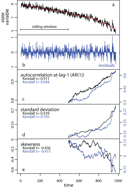
We present the rolling window metrics applied to a simulated time series in which a critical transition is approaching (fig 1a). We estimated autocorrelation, variance (as standard deviation), and skewness within rolling windows half the size of the time series (window size=485 points). We did both on the original time series and the detrended using Gaussian smoothing with bandwidth size 10% of the time series length. We used a sliding (overlapping) moving window based on the idea that indicators should be estimated as data are becoming available. Autocorrelation at-lag-1 increases up to the transition with a strong trend as estimated by Kendall’s τ (rank correlation) both for the original (τ=0.911) and the residual (after detrending) time series (τ=0.944) (fig 1b). Standard deviation also increases in both original and detrended time series (fig 1c), while skewness generally decreases (τ = -0.436 for the original time series, τ = -0.475 for the residuals after detrending), but in a somewhat irregular fashion (fig 1d). Kurtosis shows no apparent trend (fig 1e).

 

 

 

 

 

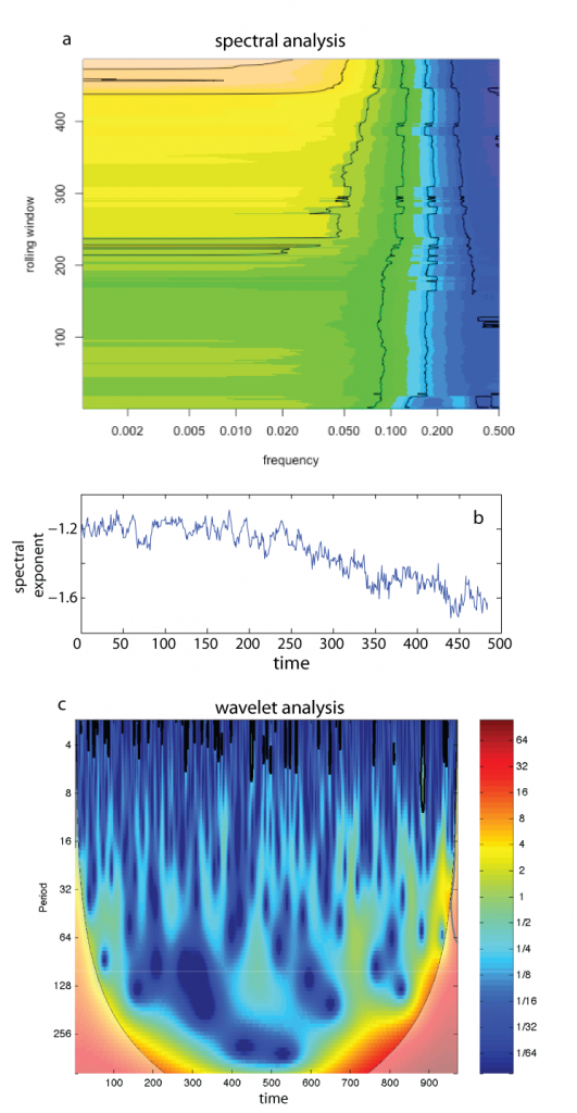
We can also get a more complete picture of the changes in the spectral properties of the time series (fig 2). The complete powerspectrum within a rolling window shows the shift in power to lower frequencies (fig 2a) that can be quantified by a decreasing spectral exponent (fig 2b). Alternatively, we can measure the contribution and significance of all periodicities in the time series using wavelet analysis (fig 2c).